Week #2. New GDAL networking API

In this post I would like to propose the final appearance of the new GDAL networking API.

I suppose, that implementing a network functionality as a GDAL driver has the following disadvantages:

1. The concept of driver in general is to provide a "bridge" between GDAL abstraction and the real data format. There is no network format itself, because every vector format stores the network (or simply connectivity) together with spatial objects or in the separate set of layers but anyway the same format.
2. An implementation of a new GDALDataset must be generic and implement only the defined interface, while we need to add new network functionality.We will need to do a type cast if we want to use network methods of the new GDALDataset.
3. Network is usually built over the ready set of spatial data. In case of driver there is a need firstly to create a void network and then import some layers from external data sets.
4. If we inherit the GDALDataset a lot of unnecessary for networks methods, such as working with rasters, will be inherited too.
5. Some drivers, which serves as an "inner" for networking driver does not support several layers, such as GeoJSON, so there is no capability to create a network over them, while this requires several layers.
6. I also suppose that some mechanisms of network model extensions, which I've implement in my driver are a bit excess and I think it is unnecessary to include it into GDAL library.

Solution

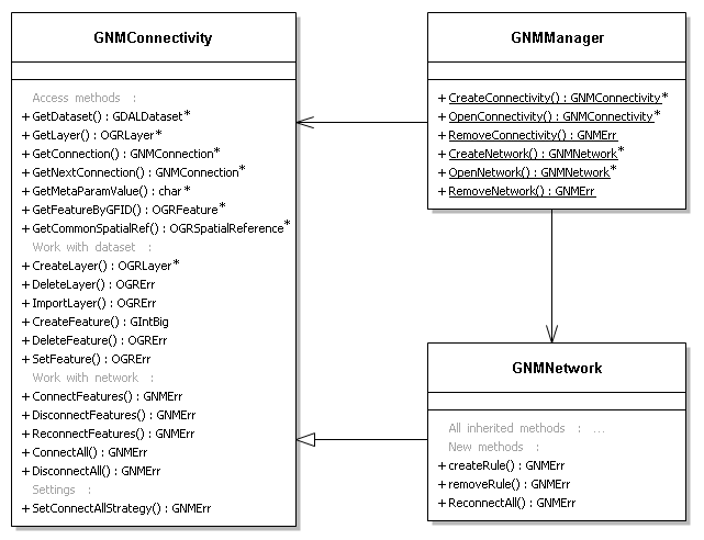
The separate class GNMConnectivity represents a network as an object and aggregates a GDALDataset instance, but not inherits it. The network data and spatial/attribute in fact are not separable (just additional layers or fields), while the GNMConnectivity "knows" which data from the data set refers to network data and operates it. The network can be built only over the existing data set (though, it can be void), wrapping it and adding missing network layers/field.

All network functionality in GDAL will be split to two levels: GNMConnectivity (level 0) and GNMNetwork (level 1). The 0 level represents a simple graph (simple connectivity or topology) which holds the connections among features. The level 1 is based on the level 0 and adds the support of network's business logic. For each level the default network functionality will be provided for any GDAL-supported vector format (at first actually for several), as it is now in my driver.

The derived classes intend to provide a support of native networking of different formats as an alternative to default. Some of these formats (like pgRouting or GML) have just connectivity capabilities without any business logic support, while others (Oracle Spatial, GDF or even ArcGIS networks) have the concept of network constraints (connectivity rules, turn restrictions). The main point is that GNMConnectivity / GNMNetwork provides the generic interface for these network formats, like GDAL provides the generic interface for spatial formats.

The derived classes also define how the network data stores in its format. For example for SpatiaLite VirtualNetwork the according "driver" will write all network data to the Roads_net_data table and to corresponding NodeFrom and NodeTo columns. If use of such "driver" hadn't been selected - the corresponding network_ layers in this simple SpatiaLite data set will be created (see my previous posts about how the network is stored). Another example: in the native form the GML "driver" will write network data to the <gml::TopoComplex>, <gml::Node> and <gml::Edge>.

API

This is a set of classes with public functions, which should be used:

Take a look at detailed description of classes, methods and its parameters:https://github.com/MikhanGusev/gnm/blob/master/gnm.h

C API: https://github.com/MikhanGusev/gnm/blob/master/gnm_api.h

network2network

The following code can be an example of using GDAL network API. It is a part of possible future utility network2network which converts the networks of different formats:

void main (void)
{
    //...
    // poPGDS initialized as a PostGIS Dataset. It has spatial data and connectivity
    // over it already.
    // poShpDS initialized as a Shapefile Dataset. It has all corresponding spatial data
    // (with the same GFIDs also), or the process of network copying will fail or be incorrect.
   
    GNMConnectivity *poPGCon = GNMManager::OpenConnectivity(poPGDS,TRUE);
    if (poPGCon == NULL) return;
    
    OGRSpatialReference *poSRS = poPGCon->GetCommonSpatialRef();
    GNMConnectivity *poShpCon = GNMManager::CreateConnectivity(poShpDS,poSRS,NULL);
    if (poShpCon == NULL) return;
   
    GNMConnection *con;
    poPGCon->ResetReading();
    while ((con = poPGCon->GetNextConnection()) != NULL)
    {
        GNMErr err = poShpCon->ConnectFeatures(con->nSourceGFID,
                                               con->nTargetGFID
                                               con->nConnectorGFID
                                               con->dDirCost,
                                               con->dInvCost,
                                               con->dir);           
        delete con;
       
        if (err != GNMERR_NONE)
        {
            poShpCon->DisconnectAll();
            return;
        }
    }
   
    // The correct resources freeing.
    //...   
}

Week #1. Network's business logic

As I mentioned in one of my previous posts (http://gsoc2014gnm.blogspot.ru/2014/05/model-in-action-2-analyse-network.html) all this week I worked on network's business logic. The providing capabilities are similar, for example, to ArcGIS connectivity rules, but more general: http://resources.arcgis.com/en/help/main/10.1/#/na/002r0000000q000000/

All business logic of the network is based on the string-like rules. Each string describes the rule for the class (layer) or for the whole network. It is easy to set them and remove, while they are stored in a single non-geometry layer. When the OGRGnmDataSource::addRule() is called, this string is added to the network_rules layer and immediately built into the inner structures. The rules have an effect when the methods like OGRGnmDataSource:: connectFeatures() are called.

Now the rule syntax looks like the following (but it will be certainly widen in future):

CLASS <Class name> [COSTS <Attribute name>] 
[BEHAVES AS EMITTER | TRANSMITTER | RECEIVER]

NETWORK CONNECTS <Class name 1> WITH <Class name 2> [VIA  <Class name 3>]

[] means that these parts can be set separately in different strings;
| means that one of the operands can be used at the same time;

So, let's take a look at the example how to use rules.


// Code begins --------------------------------------------------------------------------

// Initialize the dataSrc as OGRGnmDataSource*.
// Import some layers: tanks, kolodci, lines, reshetki.
// The network is not created yet.

dataSrc->addRule("CLASS tanks BEHAVES AS EMITTER"); // String 1.
dataSrc->addRule("CLASS lines COSTS L"); // String 2.
dataSrc->addRule("NETWORK CONNECTS kolodci WITH kolodci VIA lines"); // String 3.
dataSrc->addRule("NETWORK CONNECTS tanks WITH kolodci"); // String 4.

// The inner rule structures will be built.
// Now, let's create a network.

dataSrc->connectFeatures(0, 1, -1, 0.0, 0.0); // 0 and 1 are GFIDs of the tanks layer.
// The result will be an error, while there is no connectivity rule between two features of tanks.

dataSrc->connectFeatures(145, 146, 5, 0.0, 0.0); // 145, 146 are kolodci features. 5 is lines feature.
// The corresponding record will be created in the network_graph, because of String 3.
// The costs of this connection will be the values of an "L" field of lines layer, because of String 2.

// Code ends ---------------------------------------------------------------------------


After that we can use a GNMSimpleNetworkAnalyser::resourceDestribution() method. It will firstly collect all source points (all tanks features) and create a connected component starting from them, because of a String 1.

Take a look at my github to see the source code: https://github.com/MikhanGusev/gnm

Model's architecture

Current model's architecture is the following (with the description at the project's repository https://github.com/MikhanGusev/gnm/blob/master/description.md):

But it is also a question now, how this new API will look like in GDAL. There are several ideas:
1. Leave all as it is now - there will be an OGR driver with additional non-generic OGR behavior, such as connectFeatures() method.

2. Create a set of new C API like functions. For example OGR_GMN_DS_ConnectFeatures(hD
S, ...) where there is a user's responsibility to pass hDS as OGRGmnDataSource.

3. Similar to (2), but fully object-oriented approach is to create a separate class hierarchy (like OGRSFDriver - OGRDataSource - OGRLayer). It will require the initialized data source of the spatial format. For example:

OGRDataSource *poDS;

// initialization of poDS ...

OGRNetwork *poNetwork;

poNetwork = OGRNetwork::create(poDS); // or OGRNetwork::open(poDS)

//...

poNetwork->createFeatures(...);

4.Use pseudo-SQL functions passed through the OGRDataSource::ExecuteSQL() method. For example ExecuteSQL("SELECT connectFeatures(/*...*/)")

Model in action #2. Analyse network

In this post I would like to describe the current network analysis functionality of the GDAL/OGR network model. If you want to know how this all "technically" works you could take a look at the description document at my Github.

Shortest path search

The shortest path problem is the typical routing problem of the road networks. To define the shortest path between to points we will use the shortestPath(long startGfid, long endGfid, OGRLayer *resultLayer) method of the simplenetworkanalysis.h package (which for its turn uses Dijkstra shortest path tree search algorithm). Let's create a new network as at was shown at previous post, defining the Esri Shapfile as the spatial format now. Note: I made some preparations to visualize the results and save them at the QGIS project, which can be also found at my Github. For example, I set the "kolodci" layer's labeling options so the GFIDs of this layer features are displayed (using the joining with network_features layer).

When all features are added and connected we firstly create a new layer (also shape) which will serve as a holder of the resulting path. Let's find the shortest path between features with 801 and 807 GFIDs. We pass the new layer and these GFIDs to the shortestPath() and after the calculations the new layer will be filled with the geometries of a built path (displayed in red).

That was the simple task because there is no alternative path between 801 and 807. Let's create them. We connect 816 with 802 and 819 with 806 and use the method with the same parameters again. The new shortest path will be found. This path will lie through the connection between 816 and 802, because the costs of the network's edges were formed with the line lengths (see the previous post) and this path is definitely shorter. Note, that while the two new connections are "logical" there are no real geometries under them and so they can not be displayed.

Now let's try another interesting capability of the model - features blocking. We block the 815 feature and that means that it will not be considered in the following graph tracing, like it is now removed from the graph. So the previous path becomes unavailable and the shortest path will lie through 819 and 806.

If we block then 818 feature there will be no path between 807 and 801 and the according error code will be returned.

Resource distribution

In the field of engineering networks the resource can be anything that spreads over the network (water, gas, electricity) from the emitter features, along the transmitter features, to the receiver features. So there is a task to see, which part of network is covered by resource in different situations, such as blocking (breaking) of some network elements.

The concept of rules plays the key role in the work with resource. It is proposed that all features of the class, that marked as EMITTER will “emit” the resource. Thus the resourceDestribution() method of the simplenetworkanalysis.h package can use the connected component search algorithm (the concrete implementation is a Breadth-first search) to define which (line) features are connected to these emitters, that means that they have a resource. Let's open our previous network and make some preparations before the resource can be collected. 

We say that the three features from the layer “tanks” (marked as stars) will play the role of emitters. We connect them with the nearest features: 0 with 807, 2 with 721 and 1 with 717. Now let's create the resulting layer and pass it to the resourceDestribution(). This layer will be filled with the features, showing the resource spreading from the multiple emitters.

Let's imagine that some junctions in our water network are broken. We block 720 and 718 and see that though a small part of network has no water now, the most part of it still has it. 

To resolve this “problem” we can build a temporary pipe from any place where the water persists. We connect 721 with 719 and see that the void section is now full with water.

The rule syntax and its analysis is the subject that I'm working on now. In the code of resourceDestribution() I simply pass the GFIDs of the “emitters” instead of parse the rule string and use some inner structures. The rules itself are more useful and describe such things as cost assignment and allowing connections verification. So I suppose that my next steps will be the following: complete and debug all, that I have already, implement the rules support and make some good tests.

Model in action #1. Building network

In this post I would like to tell about the current status of the building and storing network capabilities in the GDAL/OGR network model. To show the progress I will use my small test application and QGIS to visualize the spatial data.

Manual network creation

We start from creating a network with defining the GIS format, in which the spatial data along with all its network data will be stored. I chose a PostGIS. Though the created void network has neither spatial nor network data there are already all system tables. We add a new point layer called "tanks" and create some features in it. The network_features table will be updated with new Global Feature Identifers (GFIDs) for these features, which were assigned automatically. Now we have a set of spatial data, but don't have any topological relations among the features.

As for code - all the time before we used only the generic methods of the OGRGnmDataSource and OGRGnmLayer, such as OGRDataSource::createLayer() or OGRLayer::createFeature(). When it's time to call the specific network's behavior we need to use a type cast. For connection we call for example OGRGnmDataSource::connectFeatures(0, 1, -1, 0.0, 0.0, 2), where parameters are:

1), 2) Source and target feature GFIDs. Now these features are vertexes in a graph.
3) Connector feature GFID. If we pass -1 it means that there is no physical feature between source and target and the connection is logical. This is an edge in a graph.
4), 5) The cost of edge from source to target (direct) and from target to source (inverse).
6) Direction of edge. 2 equals to bi-directional edge.

Now the network's graph is formed. We can see in pgAdmin that there were automatically created two system edges between the connected vertexes in the network_sysedges table.

Automatic network creation

Now we are going to build a network over the existing set of spatial data. Let's take a piece of the city's drain network, which includes one line Shapefile with pipes and two point Shapefiles with wells.

Firstly we open the created on the first step network and then import this data. An importing is similar to ogr2ogr utility, while it copies all features of the layer from the external data source to our one. The coordinates of the imported features are transformed to the global network SRS. After the successful importing there is no built network yet. We must connect the required features manually (for such big amount of features it can be too difficult) or use the automatic graph building capability. In our example set of data each line feature starts and ends geographically right at the point features (or very close to them). So we can use the GNMLinePointBuilder strategy to build the graph. We define the snap tolerance (in our case it will equal 0.00005) and pass it with the layers' ids to the strategy constructor. After the successful building we get the ready graph. Note, that during the graph building the specific cost assignment behavior was used. Thus, GNMGeometryCostConnection decorator is responsible for measuring the length of the edge feature.

Conclusion

Though, there is already some network functionality in OGR there is still much work. First of all the driver is not included in GDAL. There are also many small unfinished points in the code which must be completed, such as the correct network deletion behavior or correct working with SpatiaLite format.

But by this time we can see the following: with the help of the network model based on the OGR driver it is possible to create networks. The network is a set of layers (for PostGIS it is a set of DB tables) which exist along with spatial layers. The basis of network is a graph. It can be built over spatial data manually or automatically. In the next post I would like to show what can be done from network analysis with the built network.

Introduction

Hello everyone!

In my first posts I would like to tell about what does the model look like today and what I've done already in this field. The code and technical description can be found at my Github, so I won't concentrate on it here. In my next few posts I would like to demonstrate the network model in action, to show what can be already done from the user's point of view with the concept which I propose.